Note: Graphics and equations look better when printed.
This paper was presented in ..... magazine. It is based on a paper presented at the IEEE International Conference on Control Applications, Sept. 15-18, 1996, Dearborn, MI. Pamela Haley is with the NASA Langley Research Center in Hampton, VA 23681, email: p.j.haley@larc.nasa.gov. Don Soloway is with NASA Ames Research Center in Moffett Field, CA 94035, email: don@ptolemy.arc.nasa.gov.
Generalized Predictive Control for Active Flutter Suppression
This paper presents experimental results of a transonic wind-tunnel test that demonstrates the use of Generalized Predictive Control for flutter suppression in a subsonic wind-tunnel wing model. The Generalized Predictive Control algorithm is based on the minimization of a suitable cost function over finite costing and control horizons. The cost function minimizes not only the sum of the mean square output of the plant predictions, but also the weighted square rate of change of the control input with its input constraints. An additional term was added to the cost function to compensate for dynamics of the wing model that cause it to be invariant to low input frequencies. This characteristic results in a control surface that drifts within the specified input constraints. The augmentation to the cost function that penalizes this low frequency drift is derived and demonstrated. The initial validation of the controller uses a linear plant predictor model for the computation of the control inputs. Simulation results of the closed-loop system that were used to determine nominal ranges for the tuning parameters are presented. The generalized predictive controller based on the linear predictor model successfully suppressed the flutter for all testable Mach numbers and dynamic pressures in the transonic region in both simulation and wind-tunnel testing. The results confirm that the generalized predictive controller is robust to modeling errors.
INTRODUCTION
Typically, an aircraft’s speed and altitude are limited by an envelope that is conservatively defined to be below the flutter boundary for that wing. This envelope is designed to keep the aircraft in flight conditions in which flutter does not occur. Future aircraft may incorporate flexibility in the structural design to enhance an aircraft’s performance, increase its efficiency, or to reduce its weight and cost. An aircraft that incorporates flexibility in its design is likely to require an active flutter suppression (AFS) system to remove aeroelastic instabilities.
One type of controller tested during the wind-tunnel tests was a generalized predictive controller. Generalized Predictive Control (GPC) is a linear controller that the literature claims can control non-minimum phase plants, open-loop unstable plants, plants with variable or unknown dead time, and can systematically take into account real plant constraints in real-time [4]. GPC is robust with respect to modeling errors, over- and under-parameterization, and sensor noise [4]. An enhancement to GPC that takes into account plant nonlinearities is the Neural Generalized Predictive Controller (NGPC). NGPC bases its control laws on a nonlinear neural network model of the plant instead of a linear model. The validation of GPC for active flutter suppression presented in this paper is the beginning of a series of tests to verify the capabilities of NGPC.
In the remainder of the paper the section Experimental Setup describes the wind-tunnel wing model and its control system configuration. The next section, Generalized Predictive Control, covers the GPC algorithm and cost function. The GPC algorithm requires a model of the plant to calculate the control inputs. The section, BACT Modeling and Analysis, describes the modeling of the BACT wing model and shows the wing characteristics that led to the additional term being added to the cost function. This additional term is derived in the next section, An Augmentation to the Cost Function, and is followed by the Simulation Results section. This section demonstrates the effects of this extension to the cost function and presents simulated closed-loop responses for the best determined tuning parameters. The simulation results are followed by the Wind-Tunnel Results section that show that GPC can successfully suppress flutter for all testable Mach and dynamic pressures in the transonic region. Finally, the Conclusions and Recommendations section summarizes the results from the wind-tunnel test and suggests improvements for enhanced flutter suppression.
EXPERIMENTAL SETUP
The Benchmark Active Controls Technology (BACT) subsonic wind-tunnel wing model is one of the models in the Benchmark Models Program (BMP) at NASA Langley Research Center. The BMP includes a series of models varying in complexity which are used to study different aeroelastic phenomena and to validate different active controls techniques. The dynamics of the BACT wind-tunnel model are such that the aeroelastic instabilities are relatively benign, thus making it simpler to build safety mechanisms into the test facility to take over when a controller fails without destruction of the model. This makes the BACT wind-tunnel model an excellent candidate for testing new control techniques. Some of the interesting aeroelastic challenges exhibited by the BACT model are classical transonic flutter, shock induced instabilities, and separation induced oscillatory instabilities. The results presented in this paper consider the classical transonic flutter problem only.
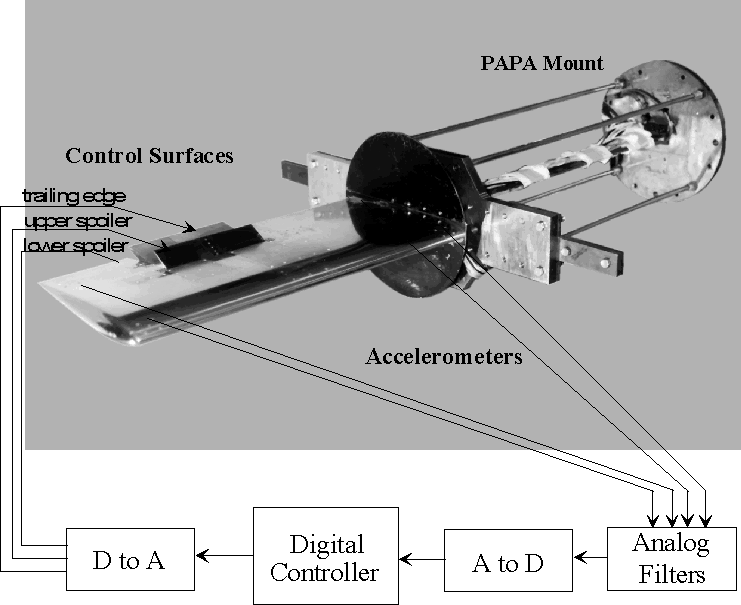
The wind-tunnel test was conducted in the Transonic Dynamics Tunnel (TDT) at NASA Langley Research Center. The TDT is capable of controlling Mach and dynamic pressure independently over a range of values [1]. The BACT wing is a rigid rectangular wing with a NACA 0012 airfoil section. It is equipped with three control surfaces (trailing-edge flap, upper-spoiler, and lower-spoiler) that are positioned by hydraulic actuators. Linear accelerometers are located one at each corner of the wing and they are used as the primary sensors for feedback control. The wing is mounted on a device called the Pitch and Plunge Apparatus (PAPA) which is designed for rotation (pitching) and vertical translation (plunging) degrees of freedom [2,3]. The characteristics of the wing and its aeroelastic properties can be set by adjustments to the PAPA mount. The BACT wing and the PAPA mount together will be referred to as the BACT plant. A wiring diagram of the BACT control system is as shown in Figure 1.
Figure 1. Wiring of BACT control system.
The accelerometer sensors are passed through a bank of 30 Hz anti-aliasing filters. These signals are sent to the digital controller after being sampled at 200 Hz. and digitized by the 12 bit analog to digital converter. The digital controller produces command signals that are sent to the digital to analog converter. These signals command the positions of the control surfaces such that minimal accelerations are produced, thus suppressing flutter. The digital controller was implemented on a Pentium Pro 150 MHz PC and the data acquisition system was the Data Translation 2839 DAQ board. Even though a Pentium Pro processor was used during the wind-tunnel tests, the control algorithm only required 4% of the CPU. This number does not include data collection and data recording. For more information on the software implementation and timing specifications refer to [7].
During the wind-tunnel tests a single-input single-output (SISO) Generalized Predictive Control system was used because the multi-input multi-output (MIMO) implementation had not been completely developed. The results reported in this paper use the inboard trailing-edge accelerometer measurements as the feedback control signal and the position of the trailing-edge flap as the control input. The BACT plant displays two aeroelastic properties, pitch and plunge. The plunge mode contributes more to the amplitude at the flutter frequency than does the pitch mode. Therefore the inboard trailing-edge accelerometer paired with the trailing-edge flap is more capable of suppressing plunge.
GENERALIZED PREDICTIVE CONTROL
Generalized Predictive Control (GPC) belongs to the class of Model-Based Predictive Control (MBPC) and was introduced by Clarke and his co-workers in 1987 [4-6]. MBPC techniques have been analyzed and implemented successfully in process control industries since the end of the 1970s and have continued to gain popularity with the increasing computational capability of computers.
The GPC system for the BACT plant is shown in Figure 2. It consists of four components: the BACT plant, a reference signal, r(n), that specifies the desired performance, a model of the plant, and the Cost Function Minimization (CFM) algorithm that determines the control surface position command needed to produce the desired performance. The principal components of the GPC algorithm are the CFM and model blocks.
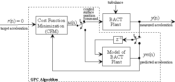
Figure 2. Block diagram of the GPC system and algorithm.
For the BACT plant the GPC was used in a regulator mode where the reference signal, r(n), was set to zero. The output of the CFM algorithm is either used as an input to the BACT plant or the BACT model. The double pole double throw switch, S, is set to the BACT plant when the CFM algorithm has solved for the best input, u(n), that will minimize a specified cost function. Between samples, the switch is set to the model where the CFM algorithm uses this model to calculate the next control input, u(n+1), from predictions of the response from the model. Once the cost function is minimized, this control input is passed to the BACT plant as a control surface position command. This algorithm is outlined below.
The GPC algorithm for the BACT plant has the following important steps.
1) Start with the previously calculated control input and predict for
the specified number of time steps the performance of the BACT plant using the model.
2) Calculate a new control input that minimizes the cost function,
3) Repeat steps 1 and 2 until desired minimization is achieved,
4) Send the first predicted control input, u(n+1), to the BACT plant,
5) Repeat the entire process for each time step.
The cost function used for the BACT plant is
![]() (1)
(1)
where
N1 is the minimum costing horizon,
N2 is the maximum costing horizon,
Nu is the control horizon,
yn is the predicted output of the model,
lu is the control input weighting
factor,
![]() is the change in u and is defined as
is the change in u and is defined as ![]() ,
,
s is the sharpness of the corners of the constraint function (see Figure 3),
upper is the upper bound of the constraint, and
lower is the lower bound of the constraint.
This cost function minimizes the sum of the mean square output of the plant predictions using a suitable plant model, weighted square of control increments, and a term which incorporates the input constraints.
The control input that best meets the constraints is produced when the cost function is minimized. This control input regulates the measured acceleration to the specified range. There are four tuning parameters in the cost function, N1, N2, Nu, and
lu. The plant’s outputs are predicted from N1 to N2 future time steps. The bound on the control horizon is Nu. The only constraint on the values of Nu and N1 is that these bounds must be less than or equal to N2. The second summation contains a weighting factor, lu, that is introduced to control the balance between the first two summations. The weighting factor acts as a damper on the next control input u(n+1). The third summation in J defines constraints placed on the control input. This constraint function is plotted in Figure 3 as the function g(u). The first two parts of the third summation form the two sides of the function while the third part insures that the function’s minimum is zero. The parameters s, upper, and lower characterize the sharpness, upper bound, and lower bound of the input constraint function, respectively. The sharpness, s, controls the shape of the constraint function. The smaller the value of s, the sharper the corners get. In practice s is set to a very small number, for example 10-20. From both the summation and Figure 3 it is easily seen that as the control input, u, approaches either the upper or lower bound, the value of the input constraint function approaches infinity.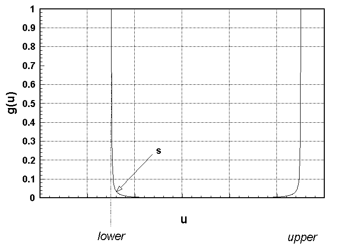
Figure 3. Plot of Input Constraint Function
A complete derivation of the GPC algorithm for a general system is developed in [7] The algorithm used to minimize the cost function is the Newton-Raphson iterative algorithm. Newton-Raphson is a quadratically converging algorithm which requires the calculation of the Jacobian and the Hessian. Although the Newton-Rhapson algorithm is computationally expensive it is justified by the low number of iterations needed for convergence. The computational issues of Newton-Rhapson are also addressed in [7].
BACT MODELING AND ANALYSIS
The GPC algorithm uses the output of the model to predict the BACT plant dynamics to an arbitrary input. With an adequate model and the correct tuning of the control parameters (N1, N2, Nu, and
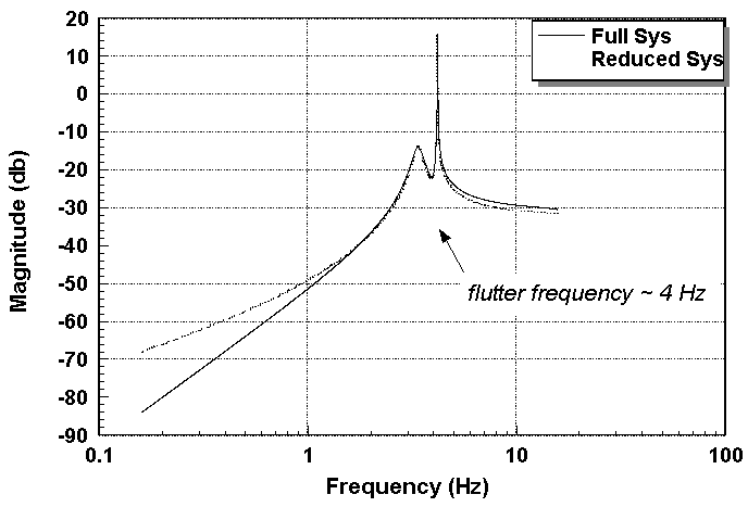
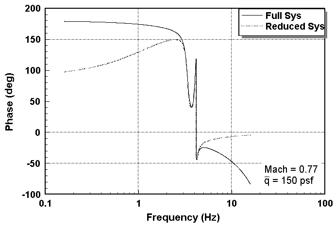
lu) the inboard trailing-edge accelerometer may be regulated to zero g’s. Since no systematic procedure exists to determine the values of these tuning parameters, the tuning of the controller can be quite cumbersome. This process could be especially difficult if tuning occurs during real-time control because each wrong choice could result in instability of the system. For this reason a GPC simulation was performed to determine the nominal ranges for the control parameters for the BACT plant. The BACT plant block, in Figure 2, was simulated using a linear model that was previously developed from the knowledge of the plant and system identification techniques using pre-existing wind-tunnel data [8]. The model of the BACT plant was a reduced order discrete model based on the model obtained in [8]. The sampling frequency for the discretization was 200 Hertz. Both models were developed for flight conditions below the flutter boundary, making them open-loop stable. The magnitude and phase plots of these models are shown in Figures 4 and 5 respectively.
|
|
Figure 4. Frequency response of the BACT models. |
Figure 5. Phase plot of BACT models. |
The reduced-order model captures the dominant modes and the dynamics
near the flutter frequency at 4 Hz., but (as seen in Figures 4 and 5) the higher order
terms have been left unmodeled. The flutter instability occurs at a dynamic pressure, ![]() , above 150 psf and a frequency around 4 Hertz.
The figures also indicate that both models have at least one zero at the origin. This
implies that the DC component and very low frequencies effectively do not pass through the
plant making the acceleration output invariant to a slow drift in the position of the
control surface. This characteristic of the plant affects the performance of the GPC
algorithm and is not accounted for in the original cost function in eq. (1). The result is
a drift in the control surface position within the specified input constraints. This
problem is also confirmed in the wind-tunnel test. The solution was to augment the cost
function with a term that penalizes a drift in the control surface position. This
enhancement is developed in the next section along with the derivation of the Jacobian and
Hessian needed for the cost function minimization. This derivation augments the derivation
found in [7].
, above 150 psf and a frequency around 4 Hertz.
The figures also indicate that both models have at least one zero at the origin. This
implies that the DC component and very low frequencies effectively do not pass through the
plant making the acceleration output invariant to a slow drift in the position of the
control surface. This characteristic of the plant affects the performance of the GPC
algorithm and is not accounted for in the original cost function in eq. (1). The result is
a drift in the control surface position within the specified input constraints. This
problem is also confirmed in the wind-tunnel test. The solution was to augment the cost
function with a term that penalizes a drift in the control surface position. This
enhancement is developed in the next section along with the derivation of the Jacobian and
Hessian needed for the cost function minimization. This derivation augments the derivation
found in [7].
AN AUGMENTATION TO THE COST FUNCTION
As mentioned in the preceding section, a low frequency drift in the control input was experienced during wind-tunnel testing. To correct this outcome, the cost function of eq. was augmented with a frequency weighted cost on the control input. The new cost function is given by
![]() (2)
(2)
where the weighted control input is the output of a discrete-time filter of the form
![]()
and l f (j) is a scalar to balance the contribution of the new term. The discrete filter, uf(n), is designed to amplify the frequencies that are to be penalized when minimizing the cost function. The design approach was to design a continuous-time high-pass filter, discretize it, and then invert the zero/pole dynamics. The resulting filter amplifies very low frequencies and the cost function minimizes them.
To include this filter in the derivation of the CFM iterative solution found in [7], the Jacobian and the Hessian of the filter are needed. Looking just at the filter part of the cost function, let
![]()
The calculation of the elements of the Jacobian are found by evaluating
![]()
and the elements of the Hessian are found by evaluating
![]()
where h and m equal 1 to Nu.
Since the filter, uf(n), is linear, its second derivative is equal to zero. This reduces the Hessian to
![]() .
.
To solve eqns. and the first derivative of the filter with respect to the input is derived and results in
![]() .
.
The first term of eq. and the second term in the summation are expanded and reduced by eliminating all derivatives equal to zero. The resulting simplifications are combined to form the conditional equation
 .
.
Equations and should be added to the Jacobian and Hessian equations of [7] for a complete solution to the GPC control input.
SIMULATION RESULTS
The GPC simulation described in the BACT Plant Analysis section was used to determine the nominal ranges for the control parameters before the wind-tunnel testing. The numerical model and the reduced order model were developed for a Mach number of 0.77 and dynamic pressure of 150 psf., a flight condition that is below the flutter boundary. The reduced order model which is in the form of an auto-regressive moving-average (ARMA) model is represented by
![]()
Since there is no systematic procedure for selecting the values of the control parameters, several experiments were conducted to find a set of control parameters that produce the smallest RMS acceleration around the flutter frequency. The four parameters N1, N2, Nu and l u took on the combinations of the values as follows: N1=1, N2, NuÎ {1,2,3,4} such that N2³ Nu; and l uÎ {0.0001, 0.001, 0.01, 0.1}. The smallest RMS value occurred when N1=1, N2=2, Nu=1 and l u=0.01.
For these simulations the relative magnitude of the control signal was constrained to ± 3 degrees to insure that the controller did not produce large deflections in the trailing-edge flap. Large deflections for flutter suppression should be avoided because the control surfaces may have physical constraints and larger deflections are typically reserved for flight control. The physical limitations in the deflection of the control surface can be incorporated in the cost function by setting the input constraint parameters accordingly. To handle this constraint the parameters s, upper and lower are set to 10-20, 3, and -3 respectively in the third summation of eq.
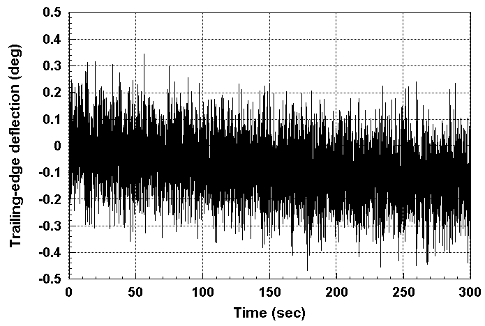
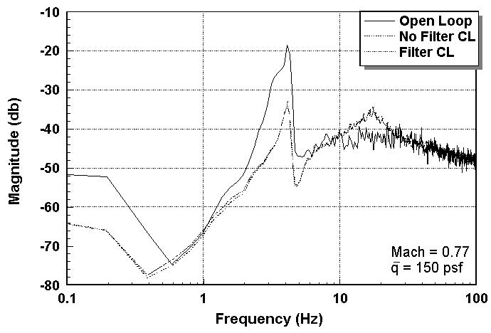
Figure 6 shows the commanded deflection of the trailing-edge flap and Figure 7 shows a comparison of the open and closed-loop response. From Figure 7, the closed-loop frequency response shows that this set of control parameters has attenuated the flutter by approximately 17 decibels. This reduction is acceptable for flutter suppression of the BACT plant and is similar to other SISO controllers tested. The control signal seen in Figure 6 shows a drift. In this simulation, the filter portion of the cost function was not activated to demonstrate the effectiveness of the filter for removing the low frequency drift.
|
|
Figure 6. Commanded control surface deflection without filter. |
Figure 7. Frequency Response of trailing-edge accelerometer. |
The filter design started with a washout filter with the transfer function
![]() .
.
The washout filter was discretized with a sampling time of 0.005 seconds using a step-invariant transform resulting in
![]() .
.
Inverting the filter we have
![]() .
.
To add this filter to the cost function set d=1 and then set the coefficient parameters to a0=1, a1=-1, b0=1, and b1=-0.995012. The filter’s weighting factor, l f, was set to 0.0001. Using this filter in the simulation yields the drift free control signal in Figure 8. The relative magnitude of the control signal has been left unchanged. The frequency response shown in Figure 9 shows that the filter has little effect on the closed-loop response.
|
|
Figure 8. Commanded control surface deflection using filter. |
Figure 9. Frequency response of trailing-edge accelerometer. |
This simulation was also tested for flight conditions above flutter. The dynamic pressure was varied from 150 psf. up to 250 psf. with Mach remaining the same at 0.77. All simulations showed similar flutter suppression capability using the same GPC system, even though the GPC system was developed for flight conditions below flutter. Therefore, the simulations results demonstrated that a fixed GPC algorithm with input constraints can provide flutter suppression for a relatively wide range of flight conditions. The robustness properties of the GPC algorithm are also confirmed with the wind-tunnel test.
WIND-TUNNEL RESULTS
During the wind-tunnel testing the same fourth-order linear ARMA model that was used during simulations was used as the model for GPC predictions. It was found that the same values for the control parameters in simulation also were the best values for control of the actual BACT plant.
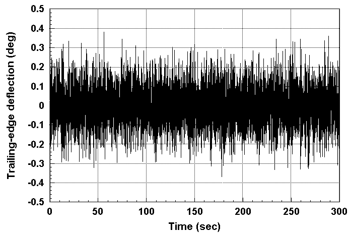
With the fixed GPC, the closed-loop system had the desirable performance characteristics. Test results without frequency weighting and control inputs constrained to ± 3 degrees are given in Figures 10 and 11. The curve in Figure 10 indicates that the input constraints are satisfied and that the command signal has the low frequency drift problem as expected. This data set represents conditions where Mach was varied from 0.75 to 0.79 and dynamic pressure was varied from 184 to 200 psf. The entire set of flight conditions were above the flutter boundary and as seen in Figure, the trailing-edge acceleration was maintained near zero throughout the test.
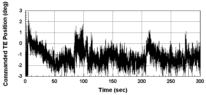
Figure 10. Commanded trailing-edge position for varying flight conditions.
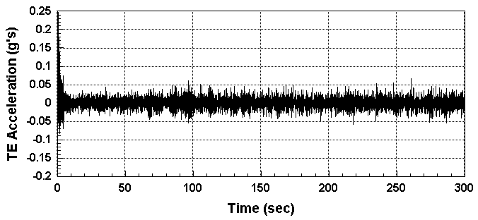
Figure 11. Accelerometer measurements for varying flight conditions.
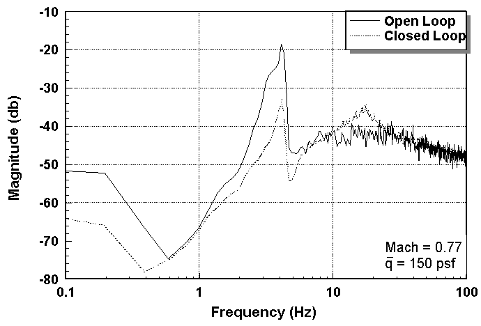
Test results with frequency weighting and input constraints set to ± 10 degrees are given in Figures 12 and 13. In this plot Mach and dynamic pressure were maintained at 0.77 and 178 psf, respectively.
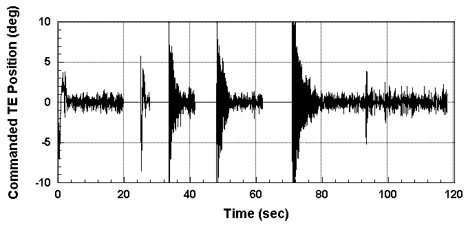
Figure 12. Commanded trailing-edge position during open- and closed-loop control.
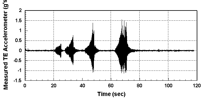
Figure 13. Accelerometer measurements during open- and closed-loop control.
The time intervals of Figure 12 with no commanded input are times when the control was allowed to go open-loop. In the corresponding time intervals in Figure 13 the accelerometer measurements start to grow. The longer the time period that the BACT plant remained uncontrolled the larger the acceleration became and the larger the commanded deflection that was needed to regain control. Notice that the control input did not contain a low frequency drift. The filter portion of the cost function was activated with l f equal to 0.0001. Since allowing a controller to go open loop during flight is not realistic, the commanded control input was set to plus and minus ten degrees to give the controller full dynamic range of the actuator.
There are several desirable control characteristics that need to be incorporated in the design of an active flutter suppression system. First, the closed-loop system must be robust to modeling errors. Next, the controller must also be able to dampen the flutter to some acceptable magnitude, within an allowable time period, and with minimal control surface deflections. In the case of the BACT plant, the damping time is not needed to be as short as with a high performance wing. Also, here the commanded inputs were only used for flutter suppression. It would be desirable for the control surface deflections to be smaller if they were also used for flight control.
CONCLUSIONS AND RECOMMENDATIONS
The results from the wind-tunnel test showed that for the tested flight conditions, the Generalized Predictive Controller was able to suppress flutter using a nominal linear model of the Benchmark Active Controls Technology plant. The wind-tunnel tests also verified that augmenting the cost function with frequency weighting on the control input is a feasible way of solving the controller’s drift problem.
To increase the flutter suppression capability of the Generalized Predictive Controller two improvements are being considered. First, a nonlinear neural network model of the Benchmark Active Controls Technology plant is being developed. This would allow the Generalized Predictive Controller to make better predictions, thus improving performance: increased flutter damping in less time and with smaller control deflections. A neural network model could also adapt to time-varying plant dynamics. A second improvement will be to use a multi-input multi-output implementation of the Generalized Predictive Controller. Using the two inboard accelerometer measurements for feedback and using the upper spoiler with the trailing-edge flap as command inputs will allow the Generalized Predictive Controller to control both plunge and pitch modes leading to enhanced flutter suppression. These improvements could lead to a shorter damping time with less control surface movement and increase the capability of the Generalized Predictive Controller to control more difficult flight conditions.
REFERENCES
[1] Aeroelasticity Branch Staff, "Langley Working Paper - The Langley Transonic Dynamics Tunnel,". NASA Langley White Paper, LWP-799, September 1969.
[2] J. A. Rivera, Jr., B. E. Dansberry, R. M. Bennett, M. H. Durham, and W. A. Silva, "NACA 0012 Benchmark Model Experimental Flutter Results with Unsteady Pressure Distributions," Proceedings of the 33rd AIAA/ ASME/ ASCE/ AHS/ ACS Structures, Structural Dynamics, and Materials Conference, AIAA Paper No. 92-2396, April 1992, Dallas, TX.
[3] J. A. Rivera, Jr., B. E. Dansberry, M. H. Durham, R. M. Bennett, and W. A. Silva, "Pressure Measurement on a Rectangular Wing with a NACA 0012 Airfoil During Conventional Flutter," NASA Technical Memorandum, TM-104211, July 1992.
[4] D. W. Clarke, C. Mohtadi and P. C. Tuffs, "Generalized Predictive Control - Part 1: The Basic Algorithm," Automatica, Volume 23, pp. 137-148, 1987.
[5] D. W. Clarke, C. Mohtadi and P. C. Tuffs, "Generalized Predictive Control - Part 2: The Basic Algorithm," Automatica, Volume 23, pp. 149-163, 1987.
[6] D. W. Clarke, "Advances in model-based predictive control," Advances in Model-Based Predictive Control, ed. by D. W. Clarke, Oxford University Press, 1994.
[7] D. Soloway and P. Haley, "Neural Generalized Predictive Control: A Newton-Raphson Implementation," Proceedings of the IEEE CCA/ISIC/CACSD, IEEE Paper No. ISIAC-TA5.2, September 15-18, 1996.
[8] M. R. Waszak, "Modeling the Benchmark Active Control Technology Wind-tunnel Model for Application to Flutter Suppression," Proceedings of the AIAA Atmospheric Flight Mechanics Conference, AIAA Paper No. 96-3437, July 29-31, 1996.